Extract selected loci¶

Synopsis¶

Pangenome graphs model the full set of genomic elements in a gives species or clade. Nevertheless, downstream analyses may require focusing on specific pangenomic regions. odgi allows to extract loci of interest from the pangenome graph, resulting in sub-graphs of the full pangenome graph. It is demonstrated that one can work with such sub-graphs as easily as handling the full ones.

Steps¶

Build the Lipoprotein A graph¶

Assuming that your current working directory is the root of the odgi project, to construct an odgi file from the LPA dataset in GFA format, execute:

odgi build -g test/LPA.gfa -o LPA.og

The command creates a file called LPA.og, which contains the input graph in odgi format. This graph contains 13 contigs from 7 haploid human genome assemblies from 6 individuals plus the chm13 cell line. The contigs cover the Lipoprotein A (LPA) locus, which encodes the Apo(a) protein.

Display path names¶

The path’s names are:

odgi paths -i LPA.og -L

chm13__LPA__tig00000001
HG002__LPA__tig00000001
HG002__LPA__tig00000005
HG00733__LPA__tig00000001
HG00733__LPA__tig00000008
HG01358__LPA__tig00000002
HG01358__LPA__tig00000010
HG02572__LPA__tig00000005
HG02572__LPA__tig00000001
NA19239__LPA__tig00000002
NA19239__LPA__tig00000006
NA19240__LPA__tig00000001
NA19240__LPA__tig00000012

Obtain the Lipoprotein A variants¶

To see the variants for the two contigs of the HG02572 sample, execute:

zgrep -v '^##' test/LPA.chm13__LPA__tig00000001.vcf.gz | head -n 9 | cut -f 1-9,16,17 | column -t

The pangenome graphs embed the full mutual relationships between the embedded genomes and their variation. In the following example, the variants were called with respect to the chm13__LPA__tig00000001 contig, which was used as the reference path.

#CHROM                   POS   ID      REF  ALT  QUAL  FILTER  INFO                        FORMAT  HG02572__LPA__tig00000001  HG02572__LPA__tig00000005
chm13__LPA__tig00000001  6     >3>6    T    A    60    .       AC=1;AF=0.5;AN=2;LV=0;NS=2  GT      1                          0
chm13__LPA__tig00000001  134   >6>8    G    GT   60    .       AC=1;AF=0.5;AN=2;LV=0;NS=2  GT      1                          0
chm13__LPA__tig00000001  156   >8>11   A    G    60    .       AC=1;AF=0.5;AN=2;LV=0;NS=2  GT      0                          1
chm13__LPA__tig00000001  252   >11>13  GT   G    60    .       AC=2;AF=1;AN=2;LV=0;NS=2    GT      1                          1
chm13__LPA__tig00000001  265   >13>16  T    A    60    .       AC=2;AF=1;AN=2;LV=0;NS=2    GT      1                          1
chm13__LPA__tig00000001  371   >16>18  AT   A    60    .       AC=2;AF=1;AN=2;LV=0;NS=2    GT      1                          1
chm13__LPA__tig00000001  996   >18>21  AG   ATT  60    .       AC=2;AF=1;AN=2;LV=0;NS=2    GT      1                          1
chm13__LPA__tig00000001  1050  >21>23  G    GT   60    .       AC=1;AF=0.5;AN=2;LV=0;NS=2  GT      1                          0

The ID field in the VCF lists the nodes involved in the variant. A > means that the node is visited in forward orientation, a < means that the node is visited in reverse orientation.

Extract a sub-graph with a variant inside¶

The insertion at position 1050 (G > GT, the last line in the VCF snippet above) is present only in one of the HG02572’s contig (HG02572__LPA__tig00000001). To extract the sub-graph where this insertion falls, execute:

odgi extract -i LPA.og -n 23 -c 1 -o LPA.21_23_G_GT.og

The instruction extracts:

The node with ID 23 (-n 23),
the nodes reachable from this node following a single edge (-c 1) in the graph topology,
the edges connecting all the extracted nodes, and
the paths traversing all the extracted nodes.

To have basic information on the sub-graph, execute:

odgi stats -i LPA.21_23_G_GT.og -S

#length nodes   edges   paths
644     5       6       3

The extracted path’s names are:

odgi paths -i LPA.21_23_G_GT.og -L

chm13__LPA__tig00000001:997-1640
HG02572__LPA__tig00000005:999-1641
HG02572__LPA__tig00000001:1035-1678

The sub-graph contains the contig used as a reference in the VCF file, and the two HG02572’s contigs.

Visualize the sub-graph¶

To visualize the sub-graph, we can also use external tools as Bandage, which supports grpahs in GFA format. To covert the graph in odgi format in a graph in GFA format, execute:

odgi view -i LPA.21_23_G_GT.og -g > LPA.21_23_G_GT.gfa

Then, open the LPA.21_23_G_GT.gfa file with Bandage.

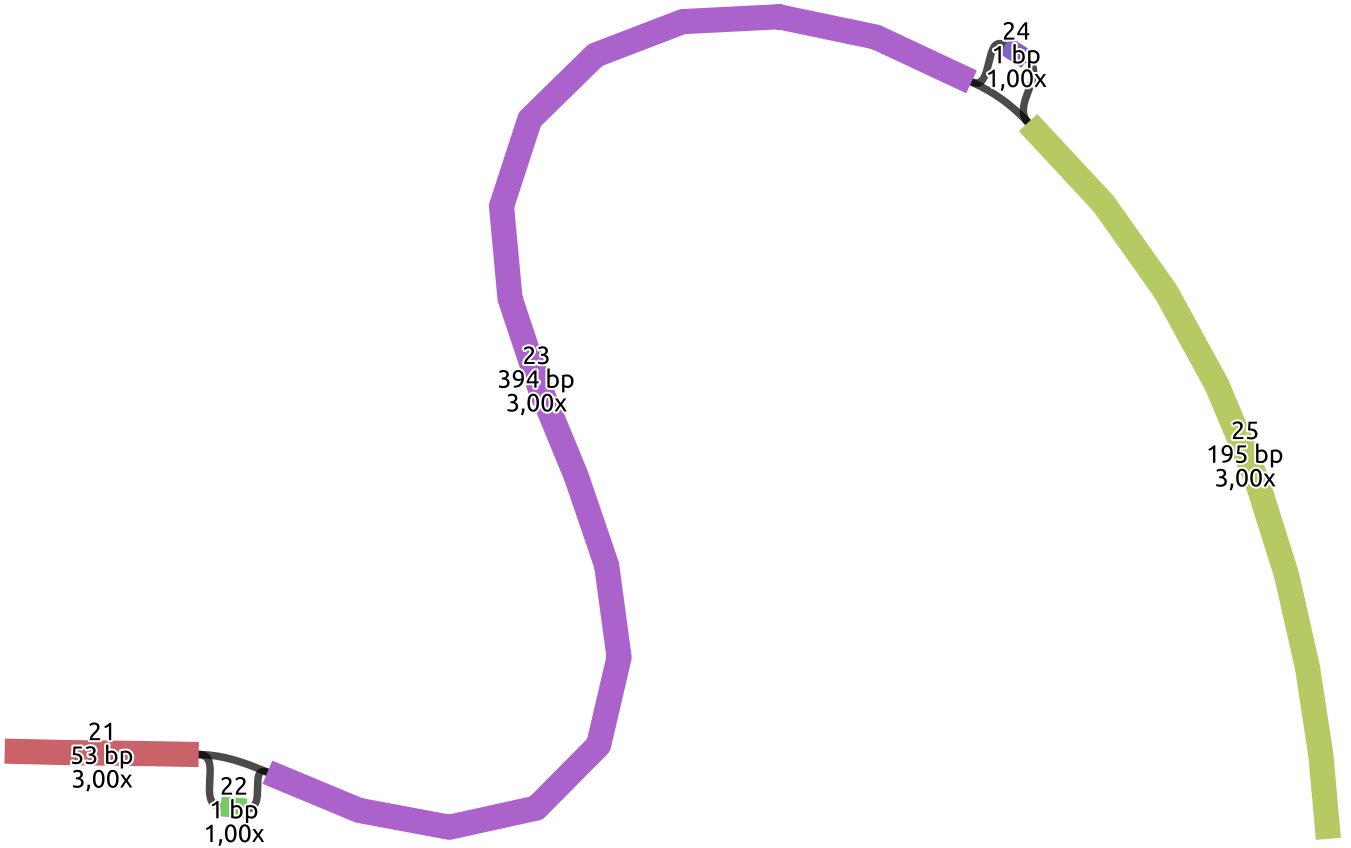
The image shows the graph topology, where each colored rectangle represents a node. In particular, three paths support nodes with ID 21 and 23, and only one path supports the node with ID 22. The node with ID 22 represents in the graph the additional nucleotide T presents in the HG02572__LPA__tig00000001 contig as an insertion.

Get the Human chr6 dataset¶

Download the pangenome graph of the Human chromosome 6 in GFA format, decompress it, and convert it to a graph in odgi format:

wget -c https://s3-us-west-2.amazonaws.com/human-pangenomics/pangenomes/scratch/2021_05_06_pggb/gfas/chr6.pan.gfa.gz
gunzip chr6.pan.gfa.gz

odgi build -g chr6.pan.gfa -o chr6.pan.og --threads 2 -P

The last command creates a file called chr6.pan.og, which contains the input graph in odgi format. This graph contains contigs of 88 haploid, phased human genome assemblies from 44 individuals, plus the chm13 and GRCh38 reference genomes.

Extract the MHC locus¶

The major histocompatibility complex (MHC) is a large locus in vertebrate DNA containing a set of closely linked polymorphic genes that code for cell surface proteins essential for the adaptive immune system. In humans, the MHC region occurs on chromosome 6. The human MHC is also called the HLA (human leukocyte antigen) complex (often just the HLA).

Assuming that your current working directory is the root of the odgi project, to see the coordinates of some HLA genes, execute:

head test/chr6.HLA_genes.bed -n 5

grch38#chr6     29722775        29738528        HLA-F
grch38#chr6     29826967        29831125        HLA-G
grch38#chr6     29941260        29945884        HLA-A
grch38#chr6     30489509        30494194        HLA-E
grch38#chr6     31268749        31272130        HLA-C

The coordinates are expressed with respect to the GRCh38 reference genome.

Extract a sub-graph with the HLA genes¶

To extract the sub-graph containing all the HLA genes annotated in the chr6.HLA_genes.bed file, execute:

odgi extract -i chr6.pan.og -o chr6.pan.MHC.og -b chr6.HLA_genes.bed  -E --threads 2 -P

The instruction extracts:

The nodes belonging to the grch38#chr6 path ranges specified in the the chr6.HLA_genes.bed file via -b,
all nodes between the min and max positions touched by the given path ranges, also if they belong to other paths (-E),
the edges connecting all the extracted nodes, and
the paths traversing all the extracted nodes.

To have basic information on the sub-graph, execute:

odgi stats -i chr6.pan.MHC.og -S

#length     nodes   edges   paths
3896981     216352  297890  97

There are 97 paths in the sub-graph. This means that for few individuals, more than one contig covers the MHC locus.

Visualize the sub-graph¶

To visualize the sub-graph with odgi, execute:

odgi sort -i chr6.pan.MHC.og -o - -O | \
    odgi viz -i - -o chr6.pan.MHC.png -s '#' -P 20

To obtain the following PNG image:

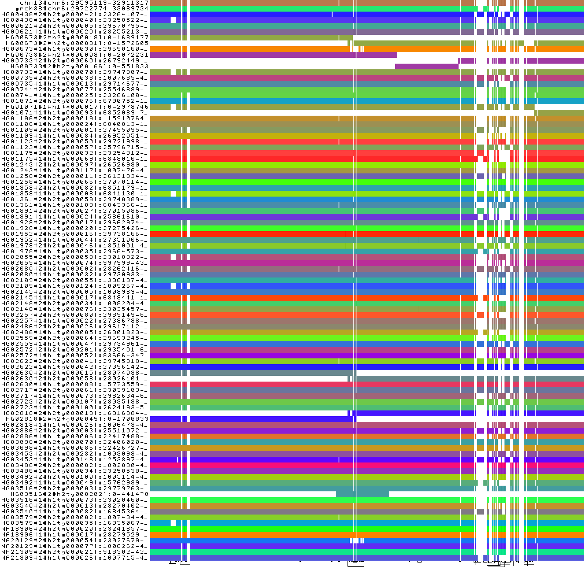
In this 1-Dimensional visualization all contigs of the same haplotype are represented with the same color (-s '#'). The majority of the haplotypes has one contig covering the whole locus, meanwhile in few of them, the locus is split in several contigs. We had to apply odgi sort here in order to optimize (-O) our sub-graph. This ensures that the node identifier space is compacted from one to the number of nodes in the sub-graph.

To see the haplotypes sorted by the number of contigs covering the MHC locus, execute:

odgi paths -i chr6.pan.MHC.og -L | cut -f 1,2 -d '#' | uniq -c | sort -k 1nr | head

HG00733#2
HG00673#2
HG01071#1
HG02630#2
HG02818#2
HG03516#2
chm13#chr6:29595119-32911317
grch38#chr6:29722774-33089734
HG00438#1
HG00438#2